Fine tuning LFM2-VL to identify car makers from images

A step by step guide on fine tuning a Vision Language Model for image identification tasks. The task we solve in this example is to identify the car maker from an image, but the learnings transfer to any other image classification task you might be interested in.

Table of Contents

• This is what you will learn
• Quickstart
• Environment setup
  • Install UV
  • Modal setup
  • Weights & Biases setup
  • Install make
• Steps
• Step 1. Dataset preparation
• Step 2. Baseline performance of LFM2-VL models
• Step 3. Structured generation to increase model robustness
• Step 4. Fine tuning with LoRA
• What's next?

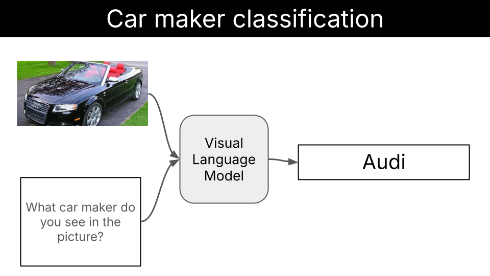
This is what you will learn

In this example, you will learn how to:

• Build a model-agnostic evaluation pipeline for vision classification tasks
• Use structured output generation with Outlines to ensure consistent and reliable model responses and increase model accuracy.
• Fine-tune a Vision Language Model with LoRA to further improve model accuracy.

Quickstart

1. Clone the repository:

git clone https://github.com/Liquid4All/cookbook.git
cd cookbook/examples/car-maker-identification

2. Evaluate base LFM2-VL models without structured generation

make evaluate config=eval_lfm_450M_raw_generation.yaml
make evaluate config=eval_lfm_1.6B_raw_generation.yaml
make evaluate config=eval_lfm_3B_raw_generation.yaml

3. Evaluate base LFM2-VL models with structured generation

make evaluate config=eval_lfm_450M_structured_generation.yaml
make evaluate config=eval_lfm_1.6B_structured_generation.yaml
make evaluate config=eval_lfm_3B_structured_generation.yaml

4. Fine-tune base LFM2-VL models with LoRA

make fine-tune config=finetune_lfm_450M.yaml
make fine-tune config=finetune_lfm_1.6B.yaml
make fine-tune config=finetune_lfm_3B.yaml

Environment setup

You will need

• uv to manage Python dependencies and run the application efficiently without creating virtual environments manually.

• Modal for GPU cloud compute. Fine-tuning a Vision Language Model without a GPU is too slow. One easy way to get access to a GPU and pay per usage is with Modal. It requires 0 infra setup and helps us get up and running with our fine-tuning experiment really fast.

• Weights & Biases (optional, but highly recommended) for experiment tracking and monitoring during fine-tuning

• make (optional) to simplify the execution of the application and fine-tuning experiments.

Let's go one by one.

Install UV

Click to see installation instructions for your platform

macOS/Linux:

curl -LsSf https://astral.sh/uv/install.sh | sh

Windows:

powershell -ExecutionPolicy ByPass -c "irm https://astral.sh/uv/install.ps1 | iex"

Modal setup

Click to see installation instructions

1. Create an account at modal.com
2. Install the Modal Python package inside your virtual environment:

   uv add modal

3. Authenticate with Modal:

   uv run modal setup

   If the first command fails, try:

   uv run python -m modal setup

Weights & Biases setup

Click to see installation instructions

1. Create an account at wandb.ai
2. Install the Weights & Biases Python package inside your virtual environment:

   uv add wandb

3. Authenticate with Weights & Biases:

   uv run wandb login

   This will open a browser window where you can copy your API key and paste it in the terminal.

Install make

Click to see installation instructions

1. Install make:

   sudo apt-get install make

Once you have installed these tools, you can git clone the repository and create the virtual environment with the following command:

git clone https://github.com/Liquid4All/cookbook.git
cd cookbook/examples/car-maker-identification
uv sync

Steps to fine-tune LFM2-VL for this task

Here's the systematic approach we follow to fine-tune LFM2-VL models for car maker identification:

1. Prepare the dataset. Collect an accurate and diverse dataset of (image, car_maker) pairs, that represents the entire distribution of inputs the model will be exposed to once deployed. You want to cover as many car makers as possible, to make sure you are never out of distribution.

2. Establish baseline performance. Evaluate pre-trained models of different sizes (450M, 1.6B, 3B) to understand current capabilities. If the results are good enough for your use case, and the model fits your deployment environment constraints, there is no need to fine tune further. Otherwise, you need to fine-tune.

3. Fine-tune with LoRA. Apply parameter-efficient fine-tuning using Low-Rank Adaptation to improve model accuracy while keeping computational costs manageable.

4. Evaluate improvements. Compare fine-tuned model performance against baselines to measure the effectiveness of our customization. If you are happy with th results, you are done. Otherwise, you need to dig deeper into model failures and improve the dataset you started with, or the fine-tuning process.

Let's go one by one.

Step 1. Dataset preparation

A fine tuned Language Model is as good as the dataset used to fine tune it

What is a good dataset for fine tuning?

A good dataset for image classification needs to be:

• Accurate: Labels must correctly match the images. For car maker identification, this means each car image is labeled with the correct manufacturer (e.g., a BMW X5 should be labeled as "BMW", not "Mercedes-Benz"). Mislabeled data will teach the model incorrect associations.

• Diverse: The dataset should represent the full range of conditions the model will encounter in production. This includes:

  • Different car models from each manufacturer
  • Various angles, lighting conditions, and backgrounds
  • Different image qualities and resolutions
  • Cars from different years and in different conditions (new, old, dirty, clean)

In this guide we will be using the Stanford Cars dataset hosted on Hugging Face.

The dataset contains:

• Classes: 49 unique car manufacturers.
• Splits: Train (6,860 images) and test (6,750 images) splits.

[TODO add barchart with class distribution]

The dataset includes additional splits with various image corruptions (gaussian noise, motion blur, etc.) for robustness testing, making it ideal for evaluating model performance under different conditions. In this tutorial we will only use the train and test splits.

Step 2. Baseline performance of LFM2-VL models

Before embarking into any fine-tuning experiment, we need to establish a baseline performance for existing models. In this case, we will evaluate the peformance of

• LFM2-VL-450M
• LFM2-VL-1.6B
• LFM2-VL-3B

To build a model-agnostic evaluation script, it is best practice to decouple the evaluation logic from the model and dataset specific code. Feel free to encapsulate the experiment parameters into any configuration file you like. One common approach is to use a YAML file, which is what we will do in this case.

In the configs directory you will find the 3 YAML files we use to evaluate these 3 models on this task

configs/
   ├── eval_lfm_450M_raw_generation.yaml
   ├── eval_lfm_1.6B_raw_generation.yaml
   └── eval_lfm_3B_raw_generation.yaml

These YAML configs are loaded into our Python script using the EvaluationConfig class in src/car_maker_identification/config.py, so we ensure

• all necessary parameters are passed and
• they all have valid values according to their types.

We use the same evaluation dataset of 100 samples, and the same system prompt and user prompt for the 3 models.

Click to see system and user prompts

system_prompt: |
  You excel at identifying car makers from pictures.

user_prompt: |
  What car maker do you see in this picture?
  Pick one from the following list:

  - AM
  - Acura
  - Aston
  - Audi
  - BMW
  - Bentley
  - Bugatti
  - Buick
  - Cadillac
  - Chevrolet
  - Chrysler
  - Daewoo
  - Dodge
  - Eagle
  - FIAT
  - Ferrari
  - Fisker
  - Ford
  - GMC
  - Geo
  - HUMMER
  - Honda
  - Hyundai
  - Infiniti
  - Isuzu
  - Jaguar
  - Jeep
  - Lamborghini
  - Land
  - Lincoln
  - MINI
  - Maybach
  - Mazda
  - McLaren
  - Mercedes-Benz
  - Mitsubishi
  - Nissan
  - Plymouth
  - Porsche
  - Ram
  - Rolls-Royce
  - Scion
  - Spyker
  - Suzuki
  - Tesla
  - Toyota
  - Volkswagen
  - Volvo
  - smart

You can run the evaluation for the 3 models with the following commands:

make evaluate config=eval_lfm_450M_raw_generation.yaml
make evaluate config=eval_lfm_1.6B_raw_generation.yaml
make evaluate config=eval_lfm_3B_raw_generation.yaml

Each evaluation run is logged as a Weights & Biases run, and you can see the results in the WandB dashboard. For each run we log 2 important metrics:

• the accuracy of the model, which is the percentage of images that the model correctly classified. This gives us a general idea of the model performance.
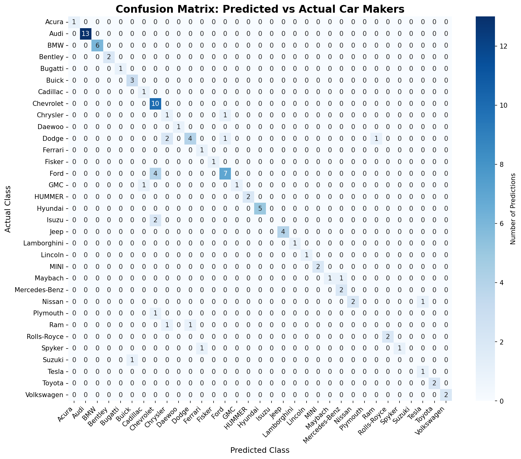
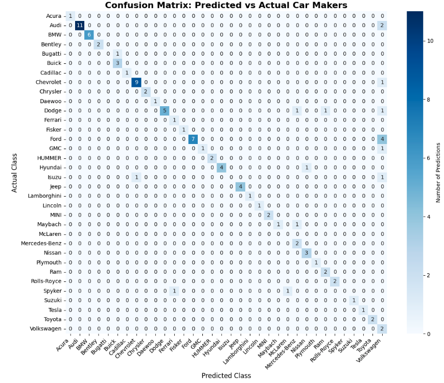
• the confusion matrix of the model. The confusion matrix is a matrix that shows the predicted labels vs the actual labels, and helps us understand better how the model performs for each class.

Baseline Results

Accuracy-wise, the 3B model is the only model that seems to work reasonably well out-of-the box, while the 450M and 1.6B models fail terribly.

Model	Accuracy
LFM2-VL-450M	3%
LFM2-VL-1.6B	0%
LFM2-VL-3B	66%

However, before blaming it on the model, let's dig deeper into the model predictions to see what's going on.

If you look at the confusion matrix of the 3B model, you will see that even though the model works okeyish overall, it sometimes fails terribly too, and generates output that does not correspond to any car maker name.

This problem is not limited to the 3B model. If you look at the confusion matrix of the 450M and 1.6B models, you will see the same pattern.

So, at this point we face the first challenge: how we "force" the model to generate outputs that are in the list of car makers?

This is what we will address in the next step.

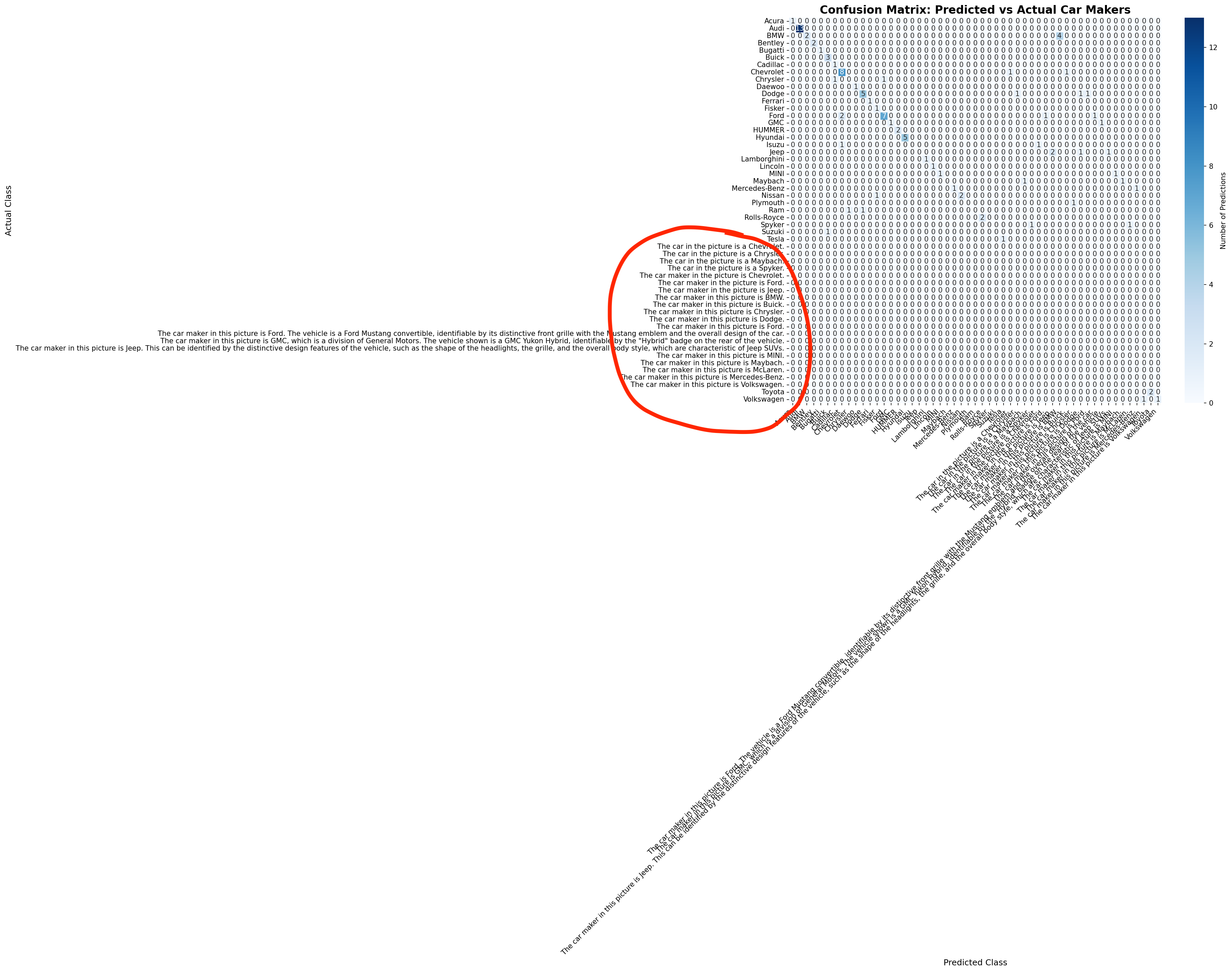
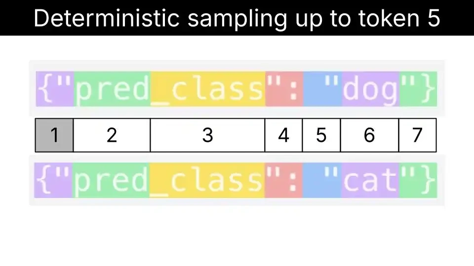
Step 3. Structured generation to increase model robustness

Structured generation is a technique that allows us to “force” the Language Model to output a specific format, like JSON, or, in our case, a valid entry from a list of car makers.

[!NOTE] Remember

Language Models generate text by sampling one token at a time. At each step of the decoding process, the model generates a probability distribution over the next token and samples one token from it.

Structured generation techniques "intervene" at each step of the decoding process, by masking tokens that are not compatible with the structured output we want to generate.

For structured generation in Python apps we recommend the Outlines library because it is easy to use, robust and well-documented.

With Outlines we define the schema of the model output and Outlines integrates with the inference provider (in this case the Transformers library) during inference to make sure that at each step of the decoding process only tokens that correspond to the schema are generated.

class CarIdentificationOutputType(BaseModel):
   pred_class: Literal[
      "AM",
      "Acura",
      "Aston",
      "Audi",
      "BMW",
      "Bentley",
      "Bugatti",
      "Buick",
      ...
      "Tesla",
      "Toyota",
      "Volkswagen",
      "Volvo",
      "smart",
   ]

The 3 configuration files to run evaluation of LFM2-VL models with structured generation are:

configs/
   ├── eval_lfm_450M_structured_generation.yaml
   ├── eval_lfm_1.6B_structured_generation.yaml
   └── eval_lfm_3B_structured_generation.yaml

You can re-run the evaluations using structured generation as follows:

make evaluate config=eval_lfm_450M_structured_generation.yaml
make evaluate config=eval_lfm_1.6B_structured_generation.yaml
make evaluate config=eval_lfm_3B_structured_generation.yaml

Structured Generation Results

Model	Accuracy
LFM2-VL-450M	58%
LFM2-VL-1.6B	74%
LFM2-VL-3B	81%

If you inspect the confusion matrix of the 3B model, you will see that the model only outputs valid car maker names, and no other text. Great!

At this point you need to decide if the performance is good enough for your use case. If it is, you are done. Otherwis, it is time to fine-tune the model.

Step 4. Fine tuning with LoRA

To fine-tune the model, we will use the LoRA technique. LoRA is a parameter-efficient fine-tuning technique that allows us to fine-tune the model by adding and tuning a small number of parameters.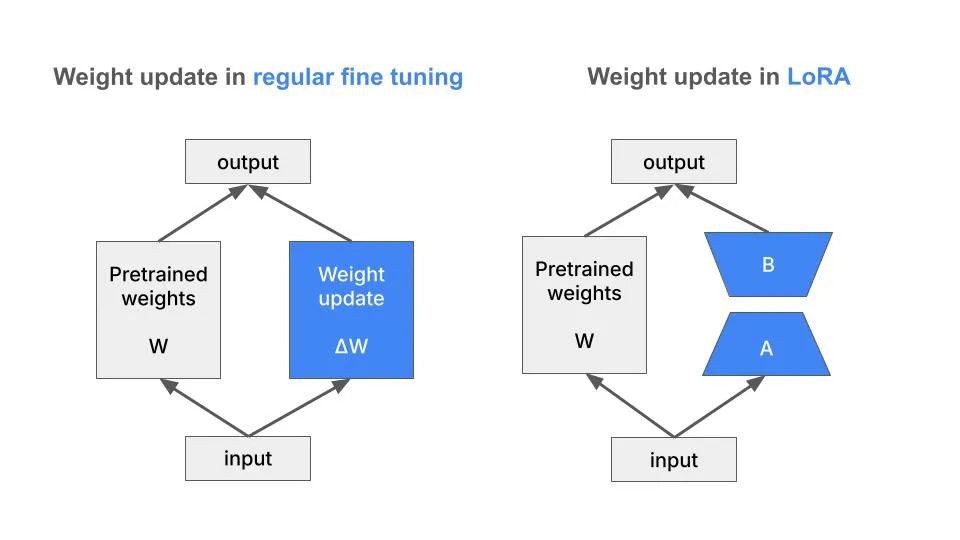

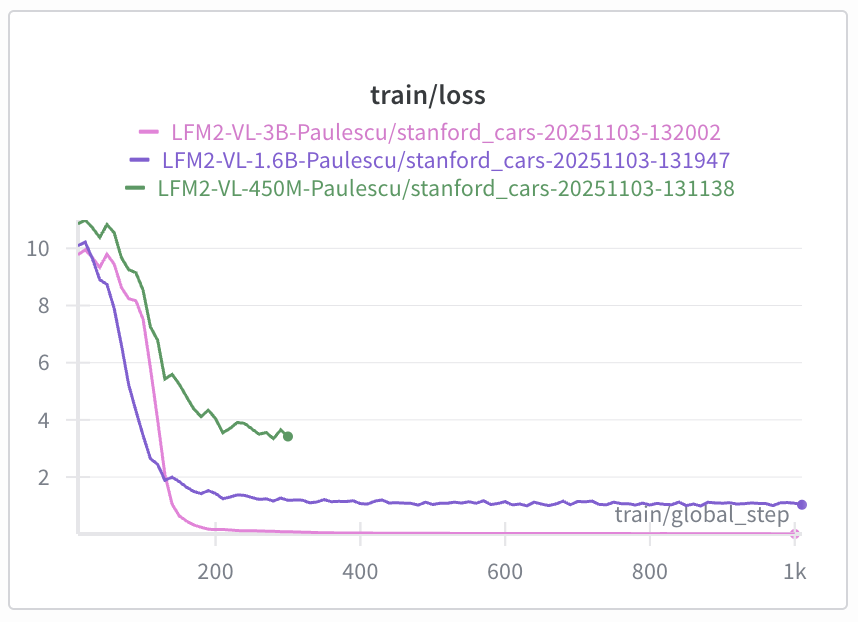
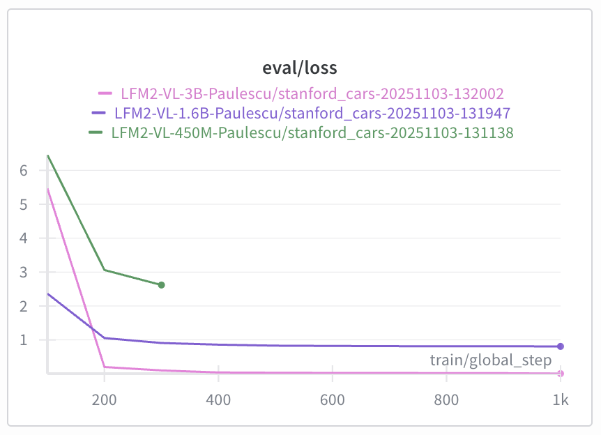
You can fine-tune each of the 3 LFM2-VL models with LoRA as follows:

make fine-tune config=finetune_lfm_450M.yaml
make fine-tune config=finetune_lfm_1.6B.yaml
make fine-tune config=finetune_lfm_3B.yaml

The train loss curves for the 3 models stabilize around very different loss values, where

• the LFM2-VL-3B model has the lowest loss, and
• the LFM2-VL-450M model has the highest loss.

At this stage we know that for the same training dataset, the LFM2-VL-3B model is able to fit the data better than the other two models.

Apart from this, the train loss curves do not tell us much about the actual model peformance. Language Models are highly parametric neural networks, that can fit anything in the training dataset. This anything includes both actual patterns in the data, and noise, that does not generalize to the test set.

So, to get a better understanding of the model performance, we need to evaluate the model on a held-out dataset. This is what the evaluation loss curve tells us.

Again LFM2-VL-3B is able to fit the data better than the other two models. When you look at its evaluation loss curve, you can see that it is stricly decreasing, meaning the model is learning epoch by epoch and still has not gotten to the point of overfitting.

The following table shows the evaluation loss at different checkpoints during fine-tuning:

Checkpoint	Train Loss	Eval Loss
100	5.82	5.46
200	0.16	0.20
300	0.07	0.10
500	0.03	0.03
1000	0.008	0.005

What is overfitting?

Overfitting is when a model learns the noise in the training data, and does not generalize to the test set. In other words, the training loss is decreasing, but the evaluation loss is increasing.

At this point, we can conclude that LFM2-VL-3B is the most promising model for our use case. However, we still need to check its actual performance on the test set.

So, let's go back to the evaluation step.

Evaluate the fine-tuned model on the test set

To evaluate the fine-tuned model, we will use the evaluate.py script again, but this time we will use the last model checkpoint.

make evaluate config=eval_lfm_3B_checkpoint_1000.yaml

Fine-tuned Model Results

Checkpoint	Accuracy
Base Model (LFM2-VL-3B)	81%
checkpoint-1000	82%

The confusion matrix for the fine-tuned model is the following:

What's next?

In this example we showed you the main steps to fine-tune a Vision Language Model for an image identification tasks.

As we said before, the quality of your final model directly depends on the quality of the dataset used for the fine-tuning.

To improve the dataset quality you can:

• Increase quality by filtering out heavily cropped, occluded, or low-quality images where the brand isn't clearly identifiable
• Increase diversity by doing data augmentation on the least represented classes.